Using AI to detect Cat and Dog pictures, with Tensorflow & Keras. (1)

Cat or Dog?

Hey everyone!

I am going to write up a few articles exposing the power of Convolutional Neural Networks in image detection. To begin with, we will attempt to recognize whether an image is a Cat or a Dog using a vanilla neural network.

Google Collab:

First I would like to recommend using google collab as you don’t need to install any pesky packages and can start your AI journey right away. All you need is a Gmail account, to follow this link and click File-> new notebook.

Once you create a new file press Edit -> NoteBook settings and using the drop-down menu choose the GPU hardware accelerator. This will help speed up your TensorFlow process.

Basic google collab image.

Developing the Dataset:

First, we need to import several packages:

import numpy as np
import tensorflow_datasets as tfds
import tensorflow as tf
from tensorflow.keras import layers

Numpy will be for data manipulation, tensorflow_datasets will be used to import our dataset and we will use layers for image rescaling.

We now will import our cats_vs_dogs dataset:

totalSet = tfds.load('cats_vs_dogs', split='train', shuffle_files=True)

In this case, we want our image to be 64px by 64px. Thus we will Keras to resize each of our images to this size. Furthermore, we also want to normalize our data so our network can analyze the images quicker.

#final image size
IMG_SIZE = 64
#resize and rescale images function
resize_and_rescale =  tf.keras.Sequential([
layers.experimental.preprocessing.Resizing(IMG_SIZE, IMG_SIZE),
layers.experimental.preprocessing.Rescaling(1./127.5, offset=-1)])

Next, we want to separate our dataset into image data and corresponding labels. The labels will be “0” or “1” for cats and dogs respectively. We will also transform these arrays into NumPy arrays and resize our images.

#loop through
trainX = []
trainY = []
i = 0
for example in totalSet:
  i += 1
  print('loading %d'%(i))
  trainX.append(np.array(resize_and_rescale
  (example['image'])))
  trainY.append(np.array(example['label']))

Next, let’s transform our X and Y dataset into NumPy arrays. We will then check what the shape of our datasets will be.

#set as arrays
trainX = np.asarray(trainX)
trainY = np.asarray(trainY)
print(trainX.shape,trainY.shape)

Your output should be:

the shape of X and Y arrays

As you can see we have 20,000 photos and 20,000 corresponding labels. The X/trainX arrays each image is 64 by 64 pixels and the “3” represents the RGB color for each pixel.

Next, we want to transform our data from the RGB format to a gray image. This is simply for preference as I have no interest in color at the moment.

For RGBtoGray transformation, we simply need to transform the RGB vector to the value R*0.2126+G*0.7152+B*0.0722. This will grant us a final image shape of (20,000,64,64).

We also need to reshape our array into the shape (20,000,64*64) so each image can be inputted into our neural network. Whereby the network will train on 20,000 [64*64 = 4096] inputs.

def rgb2gray(rgb):
  return np.dot(rgb[...,:3], [0.2126, 0.7152, 0.0722])
newTrainX = []
for image in trainX:
  newTrainX.append(rgb2gray(image))
newTrainX = np.asarray(newTrainX)
newTrainX = newTrainX.reshape(newTrainX.shape[0],64*64)

Developing the Model:

We now want to develop a model capable of analyzing our dataset. First, we will import several packages:

from keras import models
from keras import layers
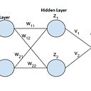
from matplotlib import pyplot

Next, we will set up a Sequential model that goes from Nodes

512 → 256 → 128 → 64 → 10 → 1

Each node will be followed by a soft plus activation layer which essentially transforms the output using the following function:

soft plus function

Graphically:

SoftPlus Graphical Function

As you can see it essentially trims off negative numbers.

The code for our network is:

#setup network
network = models.Sequential()
network.add(layers.Dense(512,input_shape=(64*64,)))
network.add(layers.Activation(tf.keras.activations.softplus))
network.add(layers.Dense(256))
network.add(layers.Activation(tf.keras.activations.softplus))
network.add(layers.Dense(128))
network.add(layers.Activation(tf.keras.activations.softplus))
network.add(layers.Dense(64))
network.add(layers.Activation(tf.keras.activations.softplus))
network.add(layers.Dense(10))
network.add(layers.Activation(tf.keras.activations.softplus))
network.add(layers.Dense(1, activation='sigmoid'))

You should notice that our last layer uses a sigmoid activation function, this is used to force our output to be between 0 and 1. This is needed since our outputs are going to be either 0 ( cat) or 1(dog). The output will thus display a probabilistic outcome (0.2 means most likely cat while 0.8 means most likely dog).

Sigmoid function

We will compile our model using the rmsprop optimizer. Since our output is binary (0 or 1) we will use binary_crossentropy loss and we will measure our accuracy.

#compile network
network.compile(optimizer='rmsprop', loss='binary_crossentropy',metrics=['accuracy'])

Finally, we will separate our data into 19000 training data and 1000 validation data. The latter will be used to analyze how good our network is with non-training data.

We will also train our system in batches of 128 and run it for 100 epochs.

val_x = newTrainX[:1000]
partial_x = newTrainX[1000:]
val_y = trainY[:1000]
partial_y = trainY[1000:]
#FIT
history =
network.fit(partial_x,partial_y,epochs=100,batch_size=128,validation_data=(val_x,val_y))

Measuring accuracy:

The history variable stores the validation accuracy and our training accuracy. The former is the accuracy with non-training data, the following code will output the maximum accuracy granted by our network with non-training data and graphical output of accuracy vs epochs.

#show loss and accuracy
#get loss for training
acc = np.asarray(history.history['accuracy'])
#get loss for testing
val_acc = np.asarray(history.history['val_accuracy'])
# x axis will display epochs running from 1 to the number of losses we have  - 1
epochs = np.asarray(range(len(acc)))
pyplot.plot(epochs,acc,'r',label='Training accuracy')
pyplot.plot(epochs,val_acc,'b',label='validation accuracy')
pyplot.title('Training and accuracy')
pyplot.xlabel('Epochs')
pyplot.ylabel('Accuracy')
pyplot.legend()
print(max(val_acc))
pyplot.show()

With our network we have the following output:

Accuracy vs Epochs (1)

We can see that the accuracy rate peaks at around 65%. This means our system recognizes cats from dogs 65% of the time which is okay but not great!

Next time we will see if we can get higher accuracy rates using a Convolutional Neural Network.

GITHUB CODE:

MoKillem/CatDogVanillaNeuralNetwork

Part 2:

Link